
Equilibrium in Goods and Money Markets
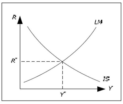
The IS–LM model explains short-run equilibrium through the intersection of two curves—IS and LM—which together determine a unique combination of interest rate and national income (GDP). At this intersection point, both the goods market and the money market are simultaneously in equilibrium. This means that total output equals total demand in the goods market, and the demand for money equals its supply in the money market. However, this equilibrium does not necessarily imply equilibrium in other sectors such as the labor market. The resulting level of income is often interpreted as the level of aggregate demand in the economy.
IS Curve (Investment–Saving Relationship)
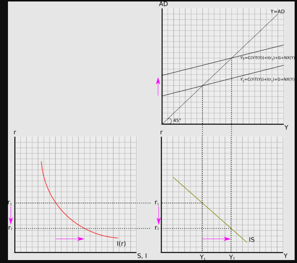
The IS curve represents equilibrium in the goods market and shows the relationship between interest rates and income. It is downward sloping because a fall in interest rates encourages investment spending, which increases total demand and raises national income. In this curve, the interest rate is treated as the independent variable, while income (GDP) is the dependent variable. The IS curve includes all combinations of interest rates and income levels where total expenditure—consisting of consumption, investment, government spending, and net exports—is equal to total output. It also reflects the condition where saving equals investment, including private saving, government saving, and foreign saving. Lower interest rates stimulate investment through cheaper borrowing, and through the multiplier effect, this leads to a larger increase in output.
Determinants of the IS Curve
The IS curve is influenced by several components of aggregate demand. Consumption depends on disposable income (income minus taxes), investment depends negatively on interest rates, government spending is determined by fiscal policy, and net exports depend on income and external factors. Any change in these components, such as an increase in government spending or a rise in exports, shifts the IS curve. The equation of the IS curve captures this relationship, showing that income is determined by consumption, investment, government expenditure, and net exports, all interacting together.
LM Curve (Liquidity–Money Relationship)

The LM curve represents equilibrium in the money market and shows combinations of interest rates and income where money demand equals money supply. It is upward sloping because higher income increases the demand for money, which in turn raises interest rates if the money supply is fixed. In this curve, income is the independent variable and the interest rate is the dependent variable. The demand for money, also called liquidity preference, depends on people’s willingness to hold cash rather than invest in interest-bearing assets.
Determinants of the LM Curve
The demand for money is determined by two main components. The first is transactions and precautionary demand, which depends positively on income because higher income leads to more spending and a need for liquidity. The second is speculative demand, which depends inversely on interest rates, as higher interest rates encourage people to hold bonds instead of cash. The supply of money, on the other hand, is determined by the central bank and is assumed to be fixed in the basic model. The LM curve is defined by the equality between real money supply and real money demand, and any increase in income shifts money demand upward, leading to higher interest rates.
Shifts in the IS Curve (Fiscal Policy Effects)
The IS curve shifts due to changes in fiscal policy or other components of demand. For example, an increase in government spending or a rise in private investment shifts the IS curve to the right, increasing both income and interest rates. Similarly, higher consumption or exports also lead to a rightward shift. Conversely, a decrease in these factors shifts the IS curve to the left. Fiscal expansion can also lead to a phenomenon known as crowding out, where higher interest rates reduce private investment. However, Keynesians argue that under certain conditions, government spending can crowd in private investment by boosting overall demand and economic growth.
Shifts in the LM Curve (Monetary Policy Effects)
The LM curve shifts due to changes in money supply or liquidity preference. An increase in the money supply shifts the LM curve to the right (or downward), leading to lower interest rates and higher income. Similarly, a decrease in liquidity preference, such as due to improved financial systems, also shifts the LM curve downward. Conversely, a decrease in money supply or an increase in liquidity preference shifts the LM curve upward, raising interest rates and reducing income.
Interaction Between IS and LM Curves
The interaction between IS and LM curves determines the equilibrium levels of income and interest rates. The effect of shifts in one curve depends on the shape of the other. For instance, if the LM curve is relatively flat, a shift in the IS curve can significantly increase income with only a small change in interest rates. On the other hand, if the LM curve is steep or vertical, the same shift may result in a large increase in interest rates with little or no change in income. This interaction is crucial in understanding the effectiveness of fiscal and monetary policies.
IS–LM Model with Interest Rate Targeting
Modern monetary policy has changed the traditional interpretation of the LM curve. Instead of controlling money supply, central banks now directly target interest rates. This has led to a modified version of the IS–LM model where the LM curve is often shown as a horizontal line, representing a fixed interest rate chosen by the central bank. This approach simplifies the model and better reflects real-world monetary policy practices. It also allows for the inclusion of inflation and expectations in the analysis.
Modern Modifications and Extensions
Economists have proposed several modifications to make the IS–LM model more realistic. For example, Olivier Blanchard introduced changes in textbooks to reflect modern monetary policy. Similarly, David Romer suggested replacing the LM curve with an MP (monetary policy) curve. John B. Taylor also contributed by emphasizing interest rate rules. These modern approaches highlight the role of central banks in directly influencing interest rates and incorporate financial factors such as risk premiums.
Conclusion
The formation of equilibrium in the IS–LM model provides a comprehensive understanding of how the goods and money markets interact to determine national income and interest rates in the short run. By analyzing shifts in the IS and LM curves, economists can study the effects of fiscal and monetary policies on the economy. Although the model has evolved over time, its core framework remains an essential tool for understanding macroeconomic equilibrium and policy impacts.