
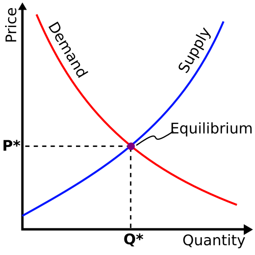
Supply and demand is a basic idea in microeconomics that explains how prices are decided in a market. It means that the price of a product depends on how much people want to buy it (demand) and how much sellers are willing to sell (supply).
In a perfectly competitive market, where many buyers and sellers exist and no one has control over prices, the price changes until it reaches a balance. This balance point is called the market equilibrium. At this point, the quantity demanded by buyers is equal to the quantity supplied by sellers.
This concept is very important because it forms the foundation of modern economics.
When Firms Have Market Power
Sometimes, markets are not perfectly competitive. In such cases, firms may have market power, which means they can influence the price.
For example, if a firm decides to produce less, it can increase the price. This breaks the basic rule of supply and demand in perfect competition.
In such situations, economists use more advanced models like:
- Oligopoly (few firms control the market)
- Differentiated product models (products are not identical)
When Buyers Have Market Power (Monopsony)
Not only sellers, but buyers can also have power in some markets. This situation is called monopsony, where a single buyer or a few buyers control the market.
In such cases, buyers can influence prices by deciding how much they want to purchase. So, the simple supply and demand model does not fully explain the market behavior here.
Supply and Demand in Macroeconomics
In macroeconomics, the idea of supply and demand is used in a broader way. Economists use the aggregate demand and aggregate supply model.
This model helps explain:
- The total output of an economy
- The overall price level
Just like in microeconomics, equilibrium occurs when total demand equals total supply.
Limitations of the Supply and Demand Model
Although supply and demand is a powerful concept, it has some limitations.
The Sonnenschein-Mantel-Debreu theorem shows that when we combine the demand of many individuals, the overall demand curve may not behave in a simple or predictable way.
This means:
- Market demand curves can take many different shapes
- The Law of Demand (price goes up → demand goes down) may not always hold true at the macro level
Because of this, it is not always guaranteed that markets will reach a stable or unique equilibrium.
Supply Schedule
A supply schedule is a table that shows the relationship between the price of a good and the quantity supplied by producers. When this relationship is shown graphically, it is called a supply curve. In a perfectly competitive market, supply depends on marginal cost, meaning firms will produce more units as long as the cost of producing an additional unit is lower than the market price.
Changes in Supply
Supply can change due to production costs. If the cost of raw materials increases, supply decreases, and the supply curve shifts to the left (or upward) because producers will supply less at each price. On the other hand, if production costs fall, supply increases, and the curve shifts to the right (or downward), meaning producers are willing to supply more at every price level.
Supply Function
Supply can also be shown using equations:
Constant Elasticity Supply Function (Curve):
Q(P) = 5P⁰·⁵
This can also be written as:
log Q(P) = log 5 + 0.5 log P
Linear Supply Function (Straight Line):
Q(P) = 3P − 6
Assumptions of Supply Curve
The supply curve assumes that firms are price takers, meaning they cannot influence market price. Each point on the curve answers the question: how much a firm will supply at a given price. However, if firms have market power (like in monopoly or oligopoly markets), they can influence prices, and the simple supply curve model no longer applies.
Individual and Market Supply
Economists distinguish between individual supply and market supply. Individual supply refers to the quantity supplied by a single firm, while market supply is the total quantity supplied by all firms in the market. Market supply is obtained by adding individual supply curves horizontally.
Short Run and Long Run Supply
Supply also differs between the short run and the long run. In the short run, some factors of production are fixed and the number of firms cannot change, so supply is less flexible. In the long run, all inputs can be adjusted and firms can enter or exit the market, making supply more responsive to price changes and generally more elastic.
Determinants of Supply
Several factors influence supply, including input prices (such as wages and raw materials), technology and productivity, expectations about future prices, and the number of suppliers in the market. These factors can shift the supply curve even when the price of the good remains the same.
Main Factors Affecting Supply
- Cost of inputs (wages, raw materials)
- Technology and productivity
- Expectations about future prices
- Number of sellers in the market
Demand Schedule
A demand schedule shows how much of a good consumers are willing and able to buy at different prices, while keeping other factors constant such as income, tastes, and prices of related goods. It is usually represented graphically as a demand curve. According to the law of demand, the demand curve is downward-sloping, which means that when the price of a product decreases, consumers tend to buy more of it. This happens because buyers will continue purchasing additional units as long as the value they get (marginal value) is higher than the price they pay.
Mathematical Representation of Demand
Demand can also be expressed using mathematical functions. A common example is a linear demand function like
Q(P) = 32 − 2P, where quantity demanded decreases as price increases.
Another form is the constant-elasticity demand function such as
Q(P) = 3P⁻², which can also be written in logarithmic form as
log Q(P) = log 3 − 2 log P.
These functions help economists understand how quantity demanded changes with price.
Graphical Representation
Traditionally, the demand curve is drawn with price on the vertical (y-axis) and quantity demanded on the horizontal (x-axis). However, in modern analysis, price is often treated as the independent variable and placed on the x-axis, while demand is shown on the y-axis. The demand curve reflects marginal utility, meaning consumers will buy a product up to the point where the utility gained equals the price paid.
Exceptions to the Law of Demand
Although demand curves usually slope downward, there are exceptions:
- Veblen goods: These are luxury goods where higher prices make them more desirable due to status or prestige.
- Giffen goods: These are inferior goods (like basic food items) where demand increases when prices rise because consumers cannot afford better alternatives. For example, when prices rise, consumers may buy more of a staple good and less of expensive items.
Individual and Market Demand
Economists distinguish between individual demand and market demand. Individual demand refers to the demand of a single consumer, while market demand is the total demand of all consumers in the market. Market demand is obtained by adding the quantities demanded by all individuals at each price level.
Determinants of Demand
Several factors influence demand apart from price. The main determinants include:
- Income of consumers
- Tastes and preferences
- Prices of related goods (substitutes and complements)
- Expectations about future prices and income
- Number of consumers in the market
- Advertising and marketing efforts
These factors can shift the demand curve either to the right (increase in demand) or to the left (decrease in demand).
History of Supply and Demand Curves
The concept of supply and demand curves has developed gradually over time, with contributions from several economists. Since both supply and demand are functions of price, they can be easily shown using graphs, which helps in better understanding market behavior.
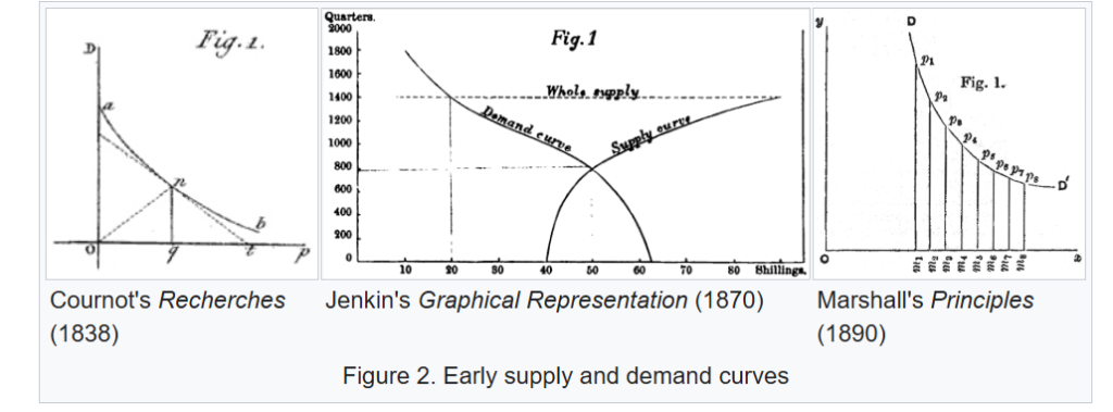
Early Contributions
The first demand curve was introduced by Augustin Cournot in 1838 in his book Recherches sur les Principes Mathématiques de la Théorie des Richesses. His work laid the foundation for representing demand as a mathematical and graphical concept.
Later, in 1870, Fleeming Jenkin added supply curves through his work on the graphical representation of supply and demand laws. This was an important step in combining both supply and demand into a single analytical framework.
Popularization by Alfred Marshall
The use of supply and demand curves became widely accepted after Alfred Marshall published Principles of Economics in 1890. Marshall refined the graphical method and made it popular in economic analysis. He also introduced the convention of showing price on the vertical axis, which is still commonly used today.
Modern Representation
When supply or demand depends on factors other than price (such as income, technology, or preferences), economists represent this using a series of curves rather than a single one. A shift from one curve to another shows changes in these other variables. In more advanced analysis, these relationships can even be represented in higher-dimensional forms.
Overall, the development of supply and demand curves has played a key role in making economic theory more visual, clear, and easier to understand.