
The XMATCH function searches for a specified item in an array or range of cells, and then returns the item’s relative position.
XMATCH Formula
=XMATCH(lookup_value, lookup_array, [match_mode], [search_mode])
| Argument | Description |
|---|---|
| lookup_value | The lookup value |
| lookup_array | The array or range to search |
| [match_mode] | 0 – Exact match (default) -1 – Exact match or next smallest item 1 – Exact match or next largest item 2 – A wildcard match where *, ?, and ~ have special meaning. |
| [search_mode] | 1 – Search first-to-last (default) -1 – Search last-to-first (reverse search). 2 – Perform a binary search that relies on lookup_array being sorted in ascending order. If not sorted, invalid results will be returned. -2 – Perform a binary search that relies on lookup_array being sorted in descending order. If not sorted, invalid results will be returned. |
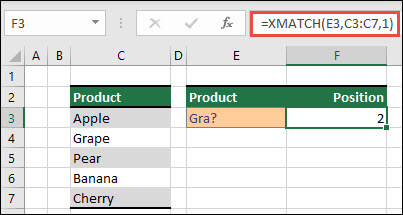
The following example finds the position of the first term that is an exact match or the next largest value for (i.e., starts with) “Gra”.
Example 2
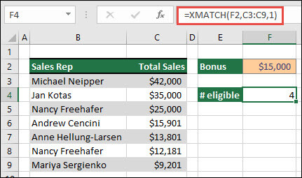
This next example finds the number of sales people eligible for a bonus. This also uses 1 for the match_mode to find an exact match or the next largest item in the list, but since the data is numeric it returns a count of values. In this case, the function returns 4, since there are 4 sales reps who exceeded the bonus amount.
Example 3
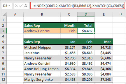
Next, we’ll use a combination of INDEX/XMATCH/XMATCH to perform a simultaneous vertical and horizontal lookup. In this case, we want to return the sales amount for a given sales rep and a given month. This is similar to using the INDEX and MATCH functions in conjunction, except that it requires fewer arguments.
Example 4
You can also use XMATCH to return a value in an array. For example, =XMATCH(4,{5,4,3,2,1}) would return 2, since 4 is the second item in the array. This is an exact match scenario, whereas =XMATCH(4.5,{5,4,3,2,1},1) returns 1, as the match_mode argument (1) is set to return an exact match or the next largest item, which is 5.