
Basic Excel Formulas
| Calculator key | Description, example | Result |
| + (Plus key) | Use in a formula to add numbers. Formula: =A1+A2 Example: =4+6+2 | 12 |
| – (Minus key) | Use in a formula to subtract numbers or to signify a negative number.Example: =18-12Example: =24*-5 (24 times negative 5) | 6-120 |
| x (Multiply key) | Use in a formula to multiply numbers. Example: =8*3 | 24 |
| ÷ (Divide key) | Use in a formula to divide one number by another. Example: =45/5 | 9 |
| % (Percent key) | Use in a formula with * to multiply by a percent. Example: =15%*20 | 3 |
| √ (square root) | Use the SQRT function in a formula to find the square root of a number. Example: =SQRT(64) | 8 |
| 1/x (reciprocal) | Use =1/n in a formula, where n is the number you want to divide 1 by.Example: =1/8 | 0.125 |
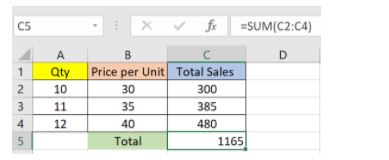
1. SUM
The SUM() function, as the name suggests, gives the total of the selected range of cell values. It performs the mathematical operation which is addition. Here’s an example of it below:
Sample Formula: “=SUM(C2:C4)”
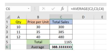
2. AVERAGE
The AVERAGE() function focuses on calculating the average of the selected range of cell values. As seen from the below example, to find the avg of the total sales, you have to simply type in:
“=AVERAGE(C2, C3, C4)”
3. COUNT
The function COUNT() counts the total number of cells in a range that contains a number. It does not include the cell, which is blank, and the ones that hold data in any other format apart from numeric.
Sample Formula: “=COUNT(C1:C4)”
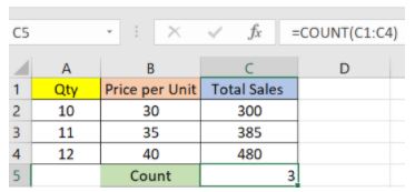
As seen above, here, we are counting from C1 to C4, ideally four cells. But since the COUNT function takes only the cells with numerical values into consideration, the answer is 3 as the cell containing “Total Sales” is omitted here.
If you are required to count all the cells with numerical values, text, and any other data format, you must use the function ‘COUNTA()’. However, COUNTA() does not count any blank cells.
To count the number of blank cells present in a range of cells, COUNTBLANK() is used.
4. SUBTOTAL
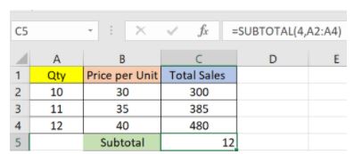
Moving ahead, let’s now understand how the subtotal function works. The SUBTOTAL() function returns the subtotal in a database. Depending on what you want, you can select either average, count, sum, min, max, min, and others. Let’s have a look at two such examples.
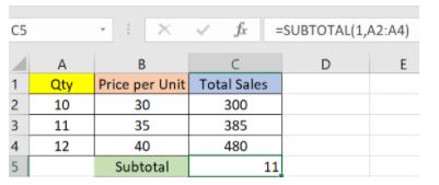
In the example above, we have performed the subtotal calculation on cells ranging from A2 to A4. As you can see, the function used is
“=SUBTOTAL(1, A2: A4)”
In the subtotal list “1” refers to average. Hence, the above function will give the average of A2: A4 and the answer to it is 11, which is stored in C5. Similarly,
“=SUBTOTAL(4, A2: A4)”
This selects the cell with the maximum value from A2 to A4, which is 12. Incorporating “4” in the function provides the maximum result.
5. MODULUS
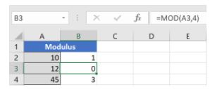
The MOD() function works on returning the remainder when a particular number is divided by a divisor. Let’s now have a look at the examples below for better understanding.
- In the first example, we have divided 10 by 3. The remainder is calculated using the function
“=MOD(A2,3)”
- The result is stored in B2. We can also directly type “=MOD(10,3)” as it will give the same answer.
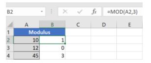
- Similarly, here, we have divided 12 by 4. The remainder is 0 is, which is stored in B3.
6. POWER
The function “Power()” returns the result of a number raised to a certain power. Let’s have a look at the examples shown below:
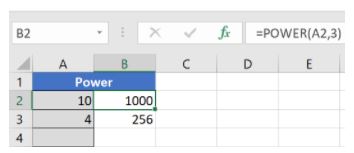
As you can see above, to find the power of 10 stored in A2 raised to 3, we have to type:
“= POWER (A2,3)”
7. CEILING
Next, we have the ceiling function. The CEILING() function rounds a number up to its nearest multiple of significance.
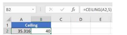
The nearest highest multiple of 5 for 35.316 is 40.
8. FLOOR
Contrary to the Ceiling function, the floor function rounds a number down to the nearest multiple of significance.
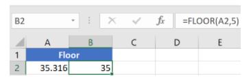
The nearest lowest multiple of 5 for 35.316 is 35.
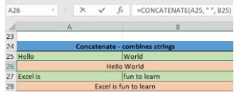
9. CONCATENATE
This function merges or joins several text strings into one text string. Given below are the different ways to perform this function.
- In this example, we have operated with the syntax:
“=CONCATENATE(A25, ” “, B25)”
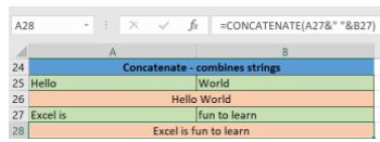
- In this example, we have operated with the syntax:
“=CONCATENATE(A27&” “&B27)”
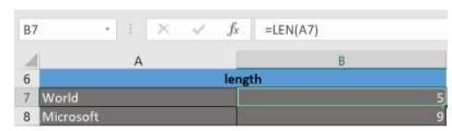
10. LEN
The function LEN() returns the total number of characters in a string. So, it will count the overall characters, including spaces and special characters. Given below is an example of the Len function.
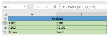
11. REPLACE
As the name suggests, the REPLACE() function works on replacing the part of a text string with a different text string.
The syntax is “=REPLACE(old_text, start_num, num_chars, new_text)”. Here, start_num refers to the index position you want to start replacing the characters with. Next, num_chars indicate the number of characters you want to replace.
Let’s have a look at the ways we can use this function.
- Here, we are replacing A101 with B101 by typing
“=REPLACE(A15,1,1,”B”)”
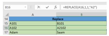
- Next, we are replacing A102 with A2102 by typing:
“=REPLACE(A16,1,1, “A2”)”
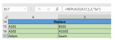
- Finally, we are replacing Adam with Saam by typing:
“=REPLACE(A17,1,2, “Sa”)”
12. SUBSTITUTE
The SUBSTITUTE() function replaces the existing text with a new text in a text string.
The syntax is “=SUBSTITUTE(text, old_text, new_text, [instance_num])”.
Here, [instance_num] refers to the index position of the present texts more than once.
Given below are a few examples of this function:
- Here, we are substituting “I like” with “He likes” by typing:
“=SUBSTITUTE(A20, “I like”,”He likes”)”
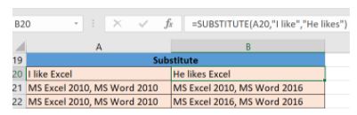
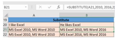
- Next, we are substituting the second 2010 that occurs in the original text in cell A21 with 2016 by typing “=SUBSTITUTE(A21,2010, 2016,2)”.
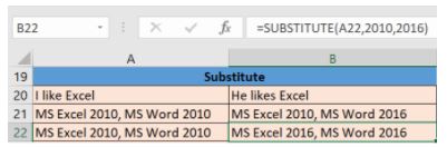
- Now, we are replacing both the 2010s in the original text with 2016 by typing “=SUBSTITUTE(A22,2010,2016)”.
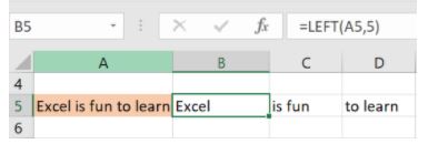
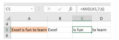
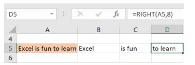
13. LEFT, RIGHT, MID
The LEFT() function gives the number of characters from the start of a text string. Meanwhile, the MID() function returns the characters from the middle of a text string, given a starting position and length. Finally, the right() function returns the number of characters from the end of a text string.
Let’s understand these functions with a few examples.
- In the example below, we use the function left to obtain the leftmost word on the sentence in cell A5.
Shown below is an example using the mid function.
- Here, we have an example of the right function.
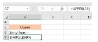
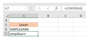
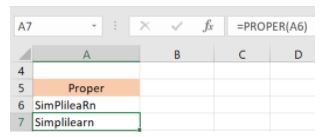
14. UPPER, LOWER, PROPER
The UPPER() function converts any text string to uppercase. In contrast, the LOWER() function converts any text string to lowercase. The PROPER() function converts any text string to proper case, i.e., the first letter in each word will be in uppercase, and all the other will be in lowercase.
Let’s understand this better with the following examples:
- Here, we have converted the text in A6 to a full uppercase one in A7.
- Now, we have converted the text in A6 to a full lowercase one, as seen in A7.
- Finally, we have converted the improper text in A6 to a clean and proper format in A7.
15. NOW()
The NOW() function in Excel gives the current system date and time.
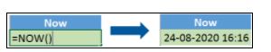
The result of the NOW() function will change based on your system date and time.
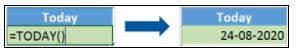
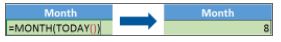
16. TODAY()
The TODAY() function in Excel provides the current system date.
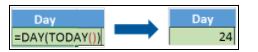
The function DAY() is used to return the day of the month. It will be a number between 1 to 31. 1 is the first day of the month, 31 is the last day of the month.
The MONTH() function returns the month, a number from 1 to 12, where 1 is January and 12 is December.
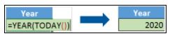
The YEAR() function, as the name suggests, returns the year from a date value.
17. TIME()
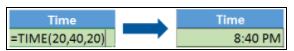
The TIME() function converts hours, minutes, seconds given as numbers to an Excel serial number, formatted with a time format.
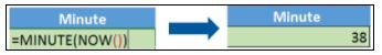
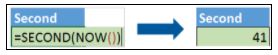
18. HOUR, MINUTE, SECOND
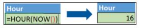
The HOUR() function generates the hour from a time value as a number from 0 to 23. Here, 0 means 12 AM and 23 is 11 PM.
The function MINUTE(), returns the minute from a time value as a number from 0 to 59.
The SECOND() function returns the second from a time value as a number from 0 to 59.
19. DATEDIF
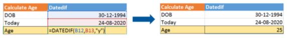
The DATEDIF() function provides the difference between two dates in terms of years, months, or days.
Below is an example of a DATEDIF function where we calculate the current age of a person based on two given dates, the date of birth and today’s date.
20. VLOOKUP
Next up in this article is the VLOOKUP() function. This stands for the vertical lookup that is responsible for looking for a particular value in the leftmost column of a table. It then returns a value in the same row from a column you specify.
Below are the arguments for the VLOOKUP function:
lookup_value – This is the value that you have to look for in the first column of a table.
table – This indicates the table from which the value is retrieved.
col_index – The column in the table from the value is to be retrieved.
range_lookup – [optional] TRUE = approximate match (default). FALSE = exact match.
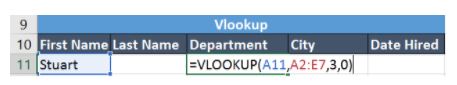
We will use the below table to learn how the VLOOKUP function works. If you wanted to find the department to which Stuart belongs, you could use the VLOOKUP function as shown below:
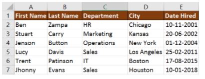
Here, A11 cell has the lookup value, A2: E7 is the table array, 3 is the column index number with information about departments, and 0 is the range lookup.
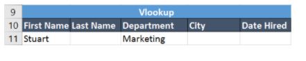
If you hit enter, it will return “Marketing”, indicating that Stuart is from the marketing department.
21. HLOOKUP
Similar to VLOOKUP, we have another function called HLOOKUP() or horizontal lookup. The function HLOOKUP looks for a value in the top row of a table or array of benefits. It gives the value in the same column from a row you specify.
Below are the arguments for the HLOOKUP function:
- lookup_value – This indicates the value to lookup.
- table – This is the table from which you have to retrieve data.
- row_index – This is the row number from which to retrieve data.
- range_lookup – [optional] This is a boolean to indicate an exact match or approximate match. The default value is TRUE, meaning an approximate match.
Given the below table, let’s see how you can find the city of Jenson using HLOOKUP.
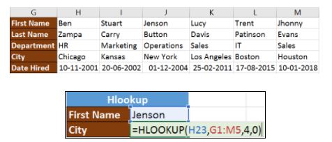
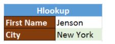
Here, H23 has the lookup value, i.e., Jenson, G1:M5 is the table array, 4 is the row index number, 0 is for an approximate match. Once you hit enter, it will return “New York”.
22. IF Formula
The IF() function checks a given condition and returns a particular value if it is TRUE. It will return another value if the condition is FALSE.
In the below example, we want to check if the value in cell A2 is greater than 5. If it’s greater than 5, the function will return “Yes 4 is greater”, else it will return “No”.
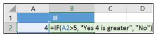
In this case, it will return ‘No’ since 4 is not greater than 5.
‘IFERROR’ is another function that is popularly used. This function returns a value if an expression evaluates to an error, or else it will return the value of the expression.
Suppose you want to divide 10 by 0. This is an invalid expression, as you can’t divide a number by zero. It will result in an error.
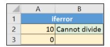
The above function will return “Cannot divide”.
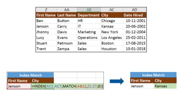
23. INDEX-MATCH
The INDEX-MATCH function is used to return a value in a column to the left. With VLOOKUP, you’re stuck returning an appraisal from a column to the right. Another reason to use index-match instead of VLOOKUP is that VLOOKUP needs more processing power from Excel. This is because it needs to evaluate the entire table array which you’ve selected. With INDEX-MATCH, Excel only has to consider the lookup column and the return column.
Using the below table, let’s see how you can find the city where Jenson resides.
Now, let’s find the department of Zampa.

24. COUNTIF
The function COUNTIF() is used to count the total number of cells within a range that meet the given condition.
Below is a coronavirus sample dataset with information regarding the coronavirus cases and deaths in each country and region.
Let’s find the number of times Afghanistan is present in the table.

The COUNTIFS function counts the number of cells specified by a given set of conditions.
If you want to count the number of days in which the cases in India have been greater than 100. Here is how you can use the COUNTIFS function.

25. SUMIF
The SUMIF() function adds the cells specified by a given condition or criteria.
Below is the coronavirus dataset using which we will find the total number of cases in India till 3rd Jun 2020. (Our dataset has information from 31st Dec 2020 to 3rd Jun 2020).

The SUMIFS() function adds the cells specified by a given set of conditions or criteria.